|
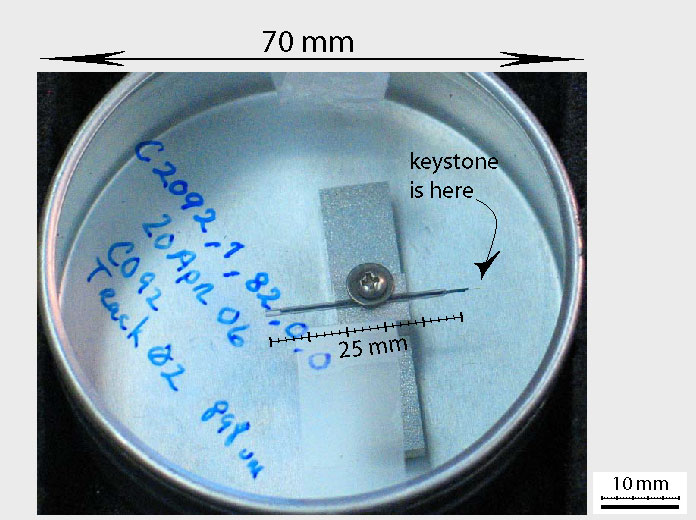
Fig. 1: Sample as received from JSC in June 2006. The track number noted in the tin is
an internal reference number and not the actual track number for
curatorial purposes.( |
|
|
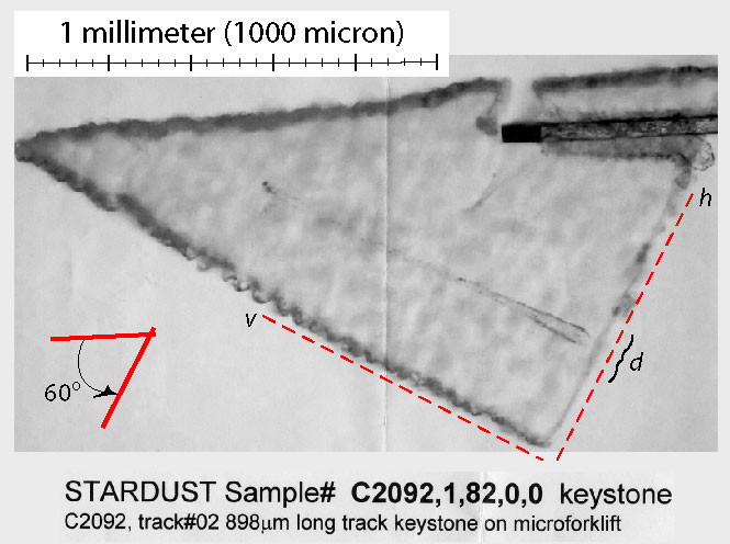
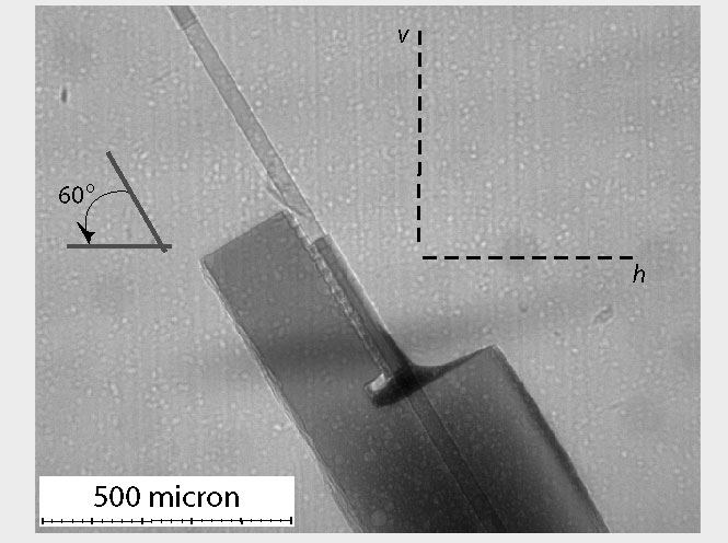
Fig. 2: Photograph of keystone. Forklift is to upper right. Angle between forklift and track is 30�.
Dashed lines indicate horizontal (h) and vertical (v) planes of tomographic volumes.
Notation d indicates entry hole depression. (photo credit Keiko Messenger, JSC, 07/06/06).
|
|
|
Fig. 4: X-ray radiograph of glass forklift/glass rod junction. Field of view 1.339 mm wide.
Inset dashed lines are vertical and horizontal directions of tomography field of view.
|
|
We obtained five tomographic data sets at 12 KeV on a 900 micron track at 1.03 and 2.06 micron/voxel edge resolution, and at three different phase contrast conditions. Images show fragment locations and track morphology. It is possible that the separate images could be combined to produce an enhanced 3D image stack. It was decided that the sample would be a good candidate for non-destructive, 2-dimensional, synchrotron x-ray fluorescence study, since particle location is known from the tomographic work.
X-normal movie (8-bit mpg, 1.7MB total).The sample was provided intact in a tin holder (Fig. 1). The keystone, by Ron (04/20/06), is sample C2092,1,82,00. The track, number 82, is 898 mm long, according to attached photo (Fig. 1). A mounting aparatus was made from clean plastics and epoxy, with a kapton window (Fig. 2). The sample container was opened in a laminar flow clean hood at APS. The forklift was used to mount the sample at an angle so that the track is vertical in the tomography aparatus (Fig. 3, 4). A small (< 1mm3) amount of plasticene clay was used to fix the glass forklift base in the hole bored in the epoxy holder base, to prevent rotation of the forklift during imaging. The kapton sleeve protecting the sample from dust was removed before run 'd', to maximize information content in the data. The sleeve was replaced immediately after the last measurement (run 'f'), before any movement of the sample. The sample was then returned to its container (Fig. 1) in the laminar flow hood.
Tomography was performed at the Advanced Photon Source (APS) at Argonne National Laboratory (Dept. Energy), on the GSECARS beamline 13 (University of Chicago), on 22-July-2006. Denton Ebel was assisted by Dr. Jon Friedrich, with students John Bigolski and Hugo Rodriquez looking on. Three entire 8 hour shifts were used to obtain five datasets at a variety of conditions. Further information on methods can be found in Ebel et al. (2006), summarized in Appendix 1.
All images were taken using a Mitutoyo 10x microscope objective, with a 100 mm extender tube, feeding a MicroMAX 5MHz camera. The field of view with this setup is 1.34 mm horizontal by 1.06 mm vertical, with ~1.03 mm/pixel edge with no binning of data.
Conditions were varied in (1) exposure time & binning, and (2) phase contrast (Table 1). All data were obtained using a 12 KeV x-ray beam. Ordinarily, data is collected on the 1300 x 1030 pixel CCD using 2x2 binning, and flat fields are collected after each 100 angles. This maximizes the signal per pixel, and reduces noise. For unbinned collection, the exposure time is roughly squared, and the number of angles must be increased (e.g., from 3 to 10 seconds from run c to run d).
Phase contrast was increased by moving the detector farther from the sample, so that beam divergence accentuated boundaries between sample regions with only subtle differences in attenuation. Three detector positions were tried: zero (minimum phase contrast, detector very close to sample), 50 mm, and 200 mm. The sample and detector geometry must be re-calibrated when the detector assembly is moved.
Resolution was limited by available hardware (extension tubes, Mitutoyo objectives), and the ability to place the objective close enough to the sample, given the location of the scintillator. Analysis of time constraints and possible improvements led to a decision not to reconfigure the existing hardware for this work. Intrinsic limits on resolution are influenced by the wavelength of visible light, properties of the scintillator, and the accuracy of the stage motor on sample rotation. Cables for x-y sample positioning, which rotate with the upper stage assembly, were removed during runs to minimize effects on rotation. In future work, we intend to use a new, more precise stage, which will eliminate some noise in sample rotation.
Results of imaging (e.g., 900 frames at ~2500kb/frame for 'd') were reconstructed using software developed by M. Rivers at GSECARS (Rivers, URL1; URL2). Parameters used were: normal, f=1.25, double corr.=1.05, averaging of flatfields, smoothing=0, air pixels=10, no ring removal, width=9.
Noise is present in all cases. Because noise in the reconstruction is higher in the center of images (the rotation center of the volume), the track in runs after 'c' was offset 300 microns with respect to the image center.
Table 1: Runs and conditions for image sets: Binning, number of angles, resolution (mm/pixel edge), detector position (mm), and exposure time (sec).| run | bin | angles | resolution | detector | exposure |
| b | 2x2 | 720 | 2.06 | 200 | 3 |
| c | 2x2 | 720 | 2.06 | 0 | 3 |
| d | 1x1 | 900 | 1.023 | 0 | 10 |
| e | 2x2 | 720 | 2.06 | 50 | 4 |
| f | 1x1 | 900 | 1.03 | 50 | 12 |
Results of reconstruction are 3D data volumes with 16-bit values for x-ray attenuation (white = higher attenuation) at each volume element (voxel). Full volume files in NetCDF format are 425 MB for binned runs, and 3.4GB for unbinned runs. The latter cannot be manipulated using IDL on a 32-bit operating system. These volumes were cropped to contain only the track, for convenience. In run 'e', for example, visual inspection establishes that the track is contained in the volume range 362 < x < 428, 230 < y < 270, and the full range of z. Cropping the volume to this range decreases its size by a factor of 10. Results are presented in two forms: MPG format movies, and stacks of TIF format images. The MPG files are compressed, and limited to 256 (8-bit) grayscales. The TIF can be output by the software as 16-bit arrays, but for the purposes here are limited to 256 bits also. Frame stacks are presented in Digital Appendix 2, the cropped volume, thresholded, is presented as Digital Appendix 3, and movies are presented in Digital Appendix 4.
The minimum and maximum values (thresholds) of the data output were set to optimize visibility of tracks and particles in the aerogel. These settings do not affect the basic volume file, but apply the full 256 grayscale range within the min/max chosen. The notation 'ts1' denotes a threshold of -1000 to +2000 grayscale values.
Successions of orthogonal track images are illustrated in Figs. 5-8. Images are numbered sequentially in the cropped volume. Each successive frame is space from the previous frame by the resolution of the imaging (e.g., 1.03 mm for 'd'), so in Fig. 5, showing every fifth frame, illustrated frames are 5.15 mm apart. The full set of images from run 'd', from which Figs. 5-7 were taken, can be found in digital form as Digital Appendix 2. These image sequences are conveniently viewed using the software 'ImageJ' (ImageJ-www), the pc port of the NIH Image software package. A set of images at the full 16-bit grayscale resolution, or at 8-bit resolution with different thresholds, can be constructed from the volume file attached as Digital Appendix 3, using the IDL routine 'tomo_display' (Rivers, URL2). Note that this software may be run in the IDL 'virtual machine' (IDL-VM, URL) without purchase of an IDL license.
Image sequences normal to the sample x-axis are included as Digital Appendix 6. Grains are indicated by arrows on these frames. These figures were made by importing 8-bit tif files from Appendix 2 into Adobe Illustrator, adding notation, and exporting as grayscale 150 dot-per-inch (dpi) tif format files. The sizes of grains has not been determined, and will require pixel-level analysis of the frames in Appendix 2. This is ongoing work.
Phase ContrastExtreme phase contrast (e.g., run 'b' at 200mm) is not useful in this case. More detailed comparison is necessary to compare runs d, e, f phase contrast). Run 'f' is not yet processed, as it requires 64-bit server to crop the volume. This work remains to be done.
BinningUnbinning was useful (compare runs d, e, f). I have focused on run 'd' as the best data set. The comparison exercise has not been done with rigor.
We have demonstrated our ability to handle fragile aerogel, and to obtain tomography data at high resolution. It might be possible to extract better information by combining data at different phase contrasts. Extreme phase contrast (e.g., run 'b' at 200mm) is not useful in this case.
We have identified many micron-sized grains in this very small track. We wish to keep this sample for non-destructive synchrotron XRF analysis. We will combine the data sets for the highest possible information return from this track, prior to extraction of the actual grains.
|
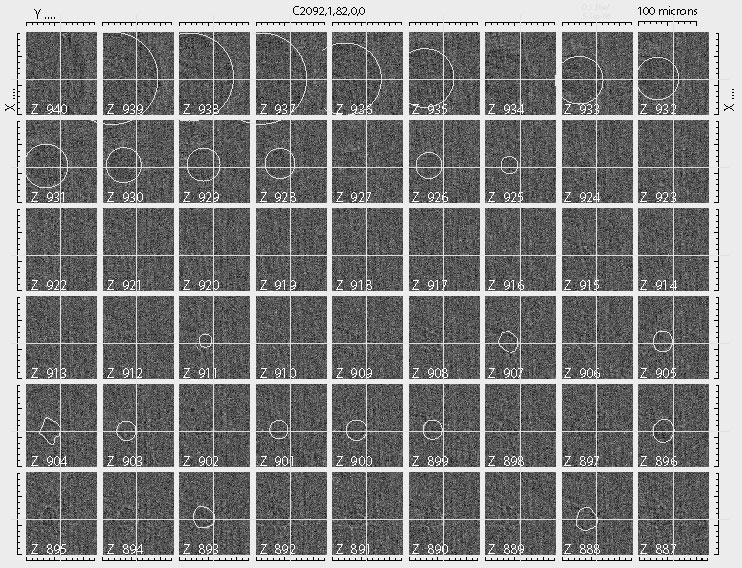
Fig. 5: Particle entry hole, in a sequence of reconstructed slices on z-axis.
Perfect circles, and irregular shapes (907, 905, 904, 893) were drawn by eye around hole
in aerogel. Grid, imposed later, lines up with inferred holes. Combined with Fig 6 and 7,
this illustrates circular depression of aerogel surface by impact (z > 924), incomplete
surface rebound (Fig. 3; Fig 6, x_40 and x_50), infilling of hole by aerogel near surface d
uring rebound (~922-917; ~5.2 mm), irregular puncturing of aerogel surface (~908-901), and
circularization of entry hole with depth (below ~988). Higher resolution: tif file. |
|
|
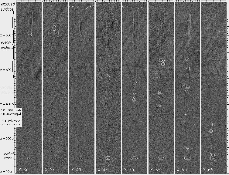
Fig. 6: Sequence of reconstructed slices on x-axis. Each fifth slice 30 through 105 is
illustrated. In rotating the sample, the tomography field of view includes the relatively
high-density glass forklift, causing artifacts in reconstruction of the aerogel+track density
structure where the forklift and track are present in the same horizontal plane (h in Fig. 2).
In frames x_40 and x_50, dashed lines indicate inferred location of aerogel surface around the
particle entry hole. Higher resolution: tif1.... tif2. FULL tif stack (zip). |
|
|
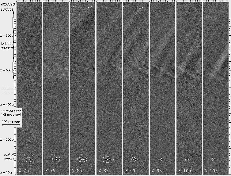
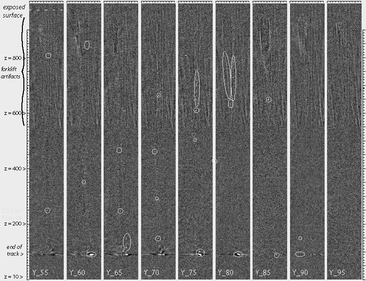
Fig. 7: Sequence of reconstructed slices on y-axis. Each fifth slice 55 through 95 is
illustrated. Higher resolution: tif file. FULL tif stack (zip). |
|
|
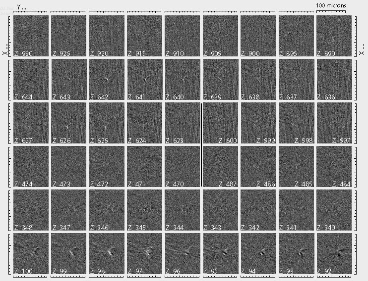
Fig. 8: Sequence of reconstructed slices on z-axis. Slices are chosen to contain the
entry hole (frames 930-890, by 5), six grains along the track, and the large terminal
particle (frames 100-92, by 1). Higher resolution: tif file. FULL tif stack (zip). |
|
|
Objective |
Digital Zoom |
Resolution |
Pixel Size |
|
Fluar 10x/0.5 |
1x |
2048x2048 |
0.45μm |
|
Fluar 20x/0.75 |
1x |
2048x2048 |
0.22μm |
|
Fluar 20x/0.75 |
2x |
2048x2048 |
0.11μm |
|
Fluar 20x/0.75 |
3x |
2048x2048 |
0.07μm |
|
Plan-Neofluar 40x/1.3 Oil |
1x |
2048x2048 |
0.11μm |
|
Plan-Neofluar 40x/1.3 Oil |
2.2x |
2048x2048 |
0.05μm |
|
Plan-Neofluar 63x/1.0 Oil |
1x |
2048x2048 |
0.07μm |
Table 1: Objective Properties
|
Scan |
Objective |
Digital Zoom |
Scan Speed / Pixel Time
(μs) |
Pinhole / Airy Units |
Detector Gain |
Number Slices |
Slice Thickness (μm) |
Laser Power (%) |
|
A - Field |
Fluar 10x/0.5 |
1x |
4 / 6.4 |
39.3 / 0.99 |
456 |
113 |
1.00 |
20.8 |
|
B - Field |
Fluar 20x/0.75 |
1x |
3 / 12.80 |
53.0 / 1.00 |
478 |
158 |
0.50 |
17.9 |
|
C - Terminal |
Fluar 20x/0.75 |
2x |
4 / 6.4 |
53.0 / 1.00 |
501 |
116 |
0.82 |
17.9 |
|
D - Entry |
Fluar 20x/0.75 |
3x |
3 / 12.80 |
48.0 / 0.91 |
419 |
199 |
0.34 |
17.9 |
|
E - Middle |
Fluar 20x/0.75 |
2x |
4 / 6.4 |
53.0 / 1.00 |
430 |
96 |
0.82 |
17.9 |
Table 2: Scan Specifics
Static images of these five scans can be seen below. (Note: these images have been resized to fit properly on the page)
|
Image 6: Scan A (10x) ... |
|
|
Image 8: Scan B (10x) ... |
|
|
Image 10: Scan C (20x) ... |
|
|
Image 12: Scan D (20x) Image may appear too dark on your screen. Increase brightness and/or
contrast to improve the image.
|
|
|
Image 14: Scan E (20x) Image may appear too dark on your screen. Increase brightness and/or
contrast to improve the image.
|
|
Full size digital images of these scans can be seen in a forthcoming Digital Appendix
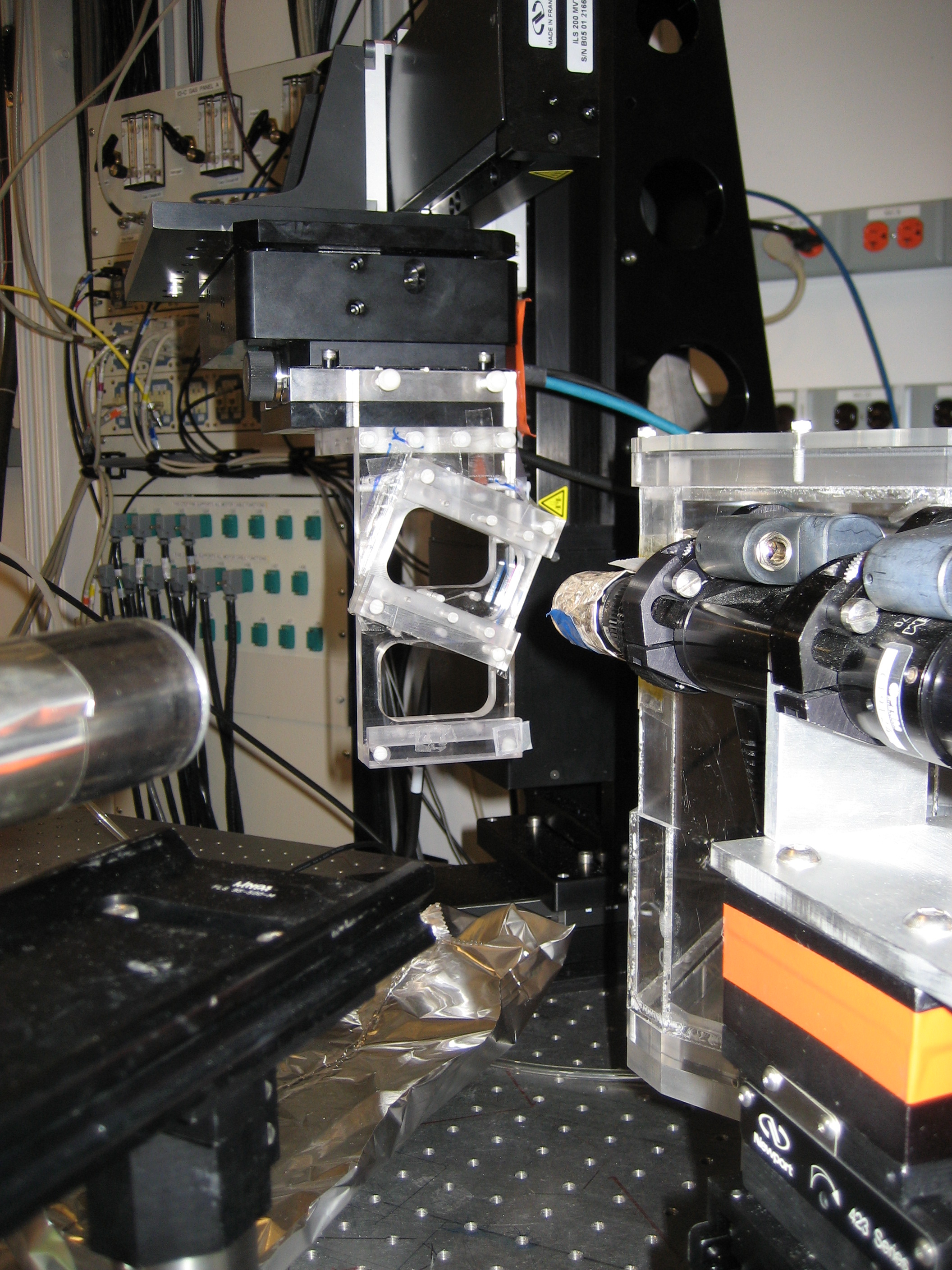
ReferencesWe performed synchrotron x-ray fluorescence mapping at the GSECARS beamline 13ID in August 2007. Resolution was 2 microns/pixel edge, for a complete map of the entire track in the keystone. The terminal particle and a large particle ~1/6 along the track are of largest size and elemental abundances could be determined with some accuracy. This XRF data has not been fully analyzed yet, however the raw data is shown below as a set of intensity maps for selected elements. These have NOT been subjected to a full spectrum analysis.
|
Setup of track holder in XRF beamline. |
|
|
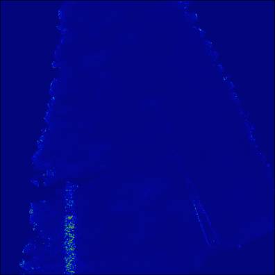
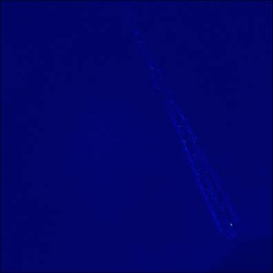
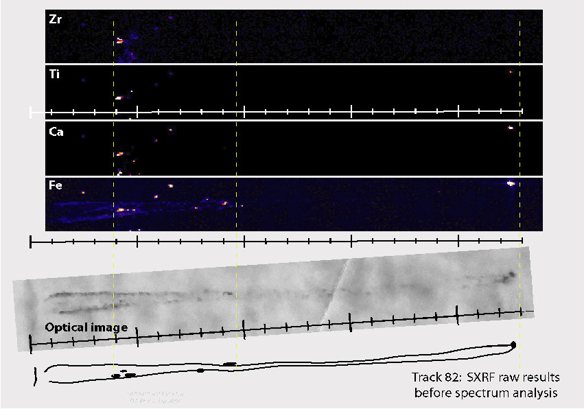
XRF raw results for Zr, Ti, Ca, Fe. Images are thresholded to emphasize the element of interest.
Dashed lines indicate locations registering optical image
of track with the XRF data. Grain at upper end of track aappears rich in Ca, Ti, and Zr.
This grain MAY BE another 'cai-like' grain. Higher resolution: tif file.... |
|
|
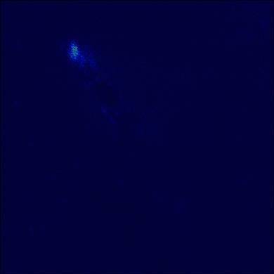
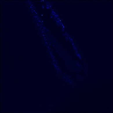
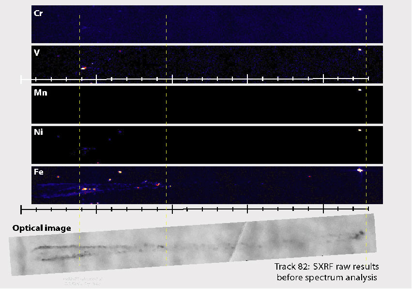
XRF raw results for Cr, V, Mn, Ni, Fe. Images are thresholded to emphasize the element of interest.
Dashed lines indicate locations registering optical image
of track with the XRF data. Terminal Particle is metal-rich. Higher resolution: tif file.... |
|