Results:
Track 82

Laser Confocal Scanning Microscopy: Technique
Technique
SM Images were taken using a Zeiss
Axiovert 100 at the Microscopy and Imaging Facility in the American Museum of
Natural History. All scans were preformed in total darkness, with all excess light
sources being sufficiently covered or switched off. The Axiovert 100 is
equipped with 4 separate laser wavelengths for analysis: 458nm Ar, 488nm Ar,
543nm HeNe, and 633nm HeNe. All data was acquired using the 488nm Ar laser to
achieve optimal resolution. The laser intensity was varied slightly with
changes in lenses, in order to preserve an acceptable amount of reflection. For
the 10x images, the laser was kept at 20.9% power, while in the 20x images, the
laser was kept at 18.9% power. Data was acquired using the Zeiss LSM 510 v.3.2
software package on a 64bit XP Intel machine. Data is collected in a
3-Dimensional array format X by Y by N, where X and Y are typical coordinates,
and N is the number of optical slices. All scans are 8bit grayscale depth at
2048x2048 resolution, and N was varied according to the relevant thickness.
8bit color depth was chosen over 12bit, due to its small difference in results,
and to optimize the size of the scan data. Once the point of best focus in a
LCSM scan is in the middle of the optical slice, all slices overlapped 1/2
or greater thickness, in order to obtain optimal clarity. Closer range images
were taken with an additional digital zoom. Unlike certain types of digital
zoom, the Axiovert 100 changes its laser scanning area, yet keeps the same scan
resolution. This allows for scans of greater magnification without any loss of
resolution or image quality. Since we used LCSM, a pinhole was used to limit
the slice thickness and limit the photons entering the detector. Our pinhole
size varied with different magnifications, but it is important to keep the
pinhole size to 1.0 Airy units or below. It is usually very difficult to take
acceptable images with a pinhole size of less than 0.9 Airy Units, due to a
lack of light passing through said pinhole. In addition, the LSM 510
software allows for Detector Gain, Amplifier Offset, and Amplifier Gain
modifiers. Amplifier Gain, and Amplifier Offset should be kept to 1.0 and 0.1
respectively, so as to reduce noise in the images. Detector Gain, however, is
the most effective means for changing the clarity of the images. A Detector
Gain value of around or below 500, allows for sufficiently clean images that
can be easily enhanced using other software packages.
When preparing to take a scan of the
aerogel, there were many constraints to keep in mind. Using the VIStting
on the microscope allows for a wider field view than the laser scans. This was
used primarily for aligning the tracks in the appropriate field of view. It is
most important to remember that when changing the field of focus the objective
is moving, and it is of the utmost importance to make sure the aerogel and
objective do not collide. The LSM 510 software gives a numerical value for the
Z height of the objective. Mapping out our maximum Z height was a crucial step
in ensuring proper data collection. Once height and spatial alignment were
determined, the microscope was switched to LSM mode, and a quick scan was
started. This allows for rapid, yet very rough scans, which can be tweaked for
optimal results. It is important to note that all microscopic parameters can be
changed on the fly during a quick scan. Also, none of the scan data from the
quick scan is saved, it is meant for alignment use only.
Furthermore, the LSM 510 software
allows for scans of variable speeds. A scan speed 3 or 4 was used, giving each
pixel on our map a scan time of 12.80μs and 6.40μs respectively.
Lower scan speeds create higher quality images, yet below scan speed 4 it is very
difficult to determine differences. Also, each line of pixels was scanned twice
and the subsequent values for each pixel averaged. This "line-mean-2"
scan method greatly improved the clarity of our images. Datasets were saved in
Zeiss' proprietary .lsm file format (a variation on regular .tiff stacks), and
were subsequently processed using Huygens Professional 3.0 (SVI) for 3D
deconvolution, and Imaris 4.5.2 64bit for display and animation techniques.
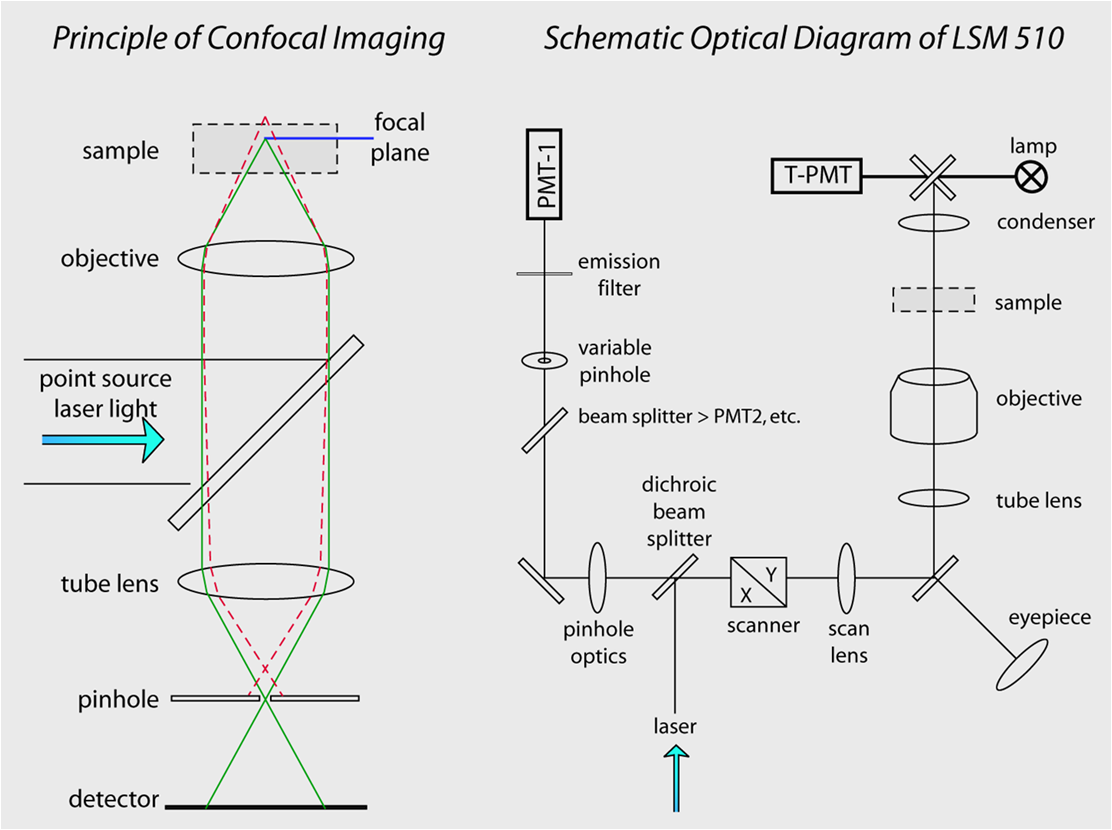
Figure 1 (left): A light path diagram for the Zeiss Axiovert 100.
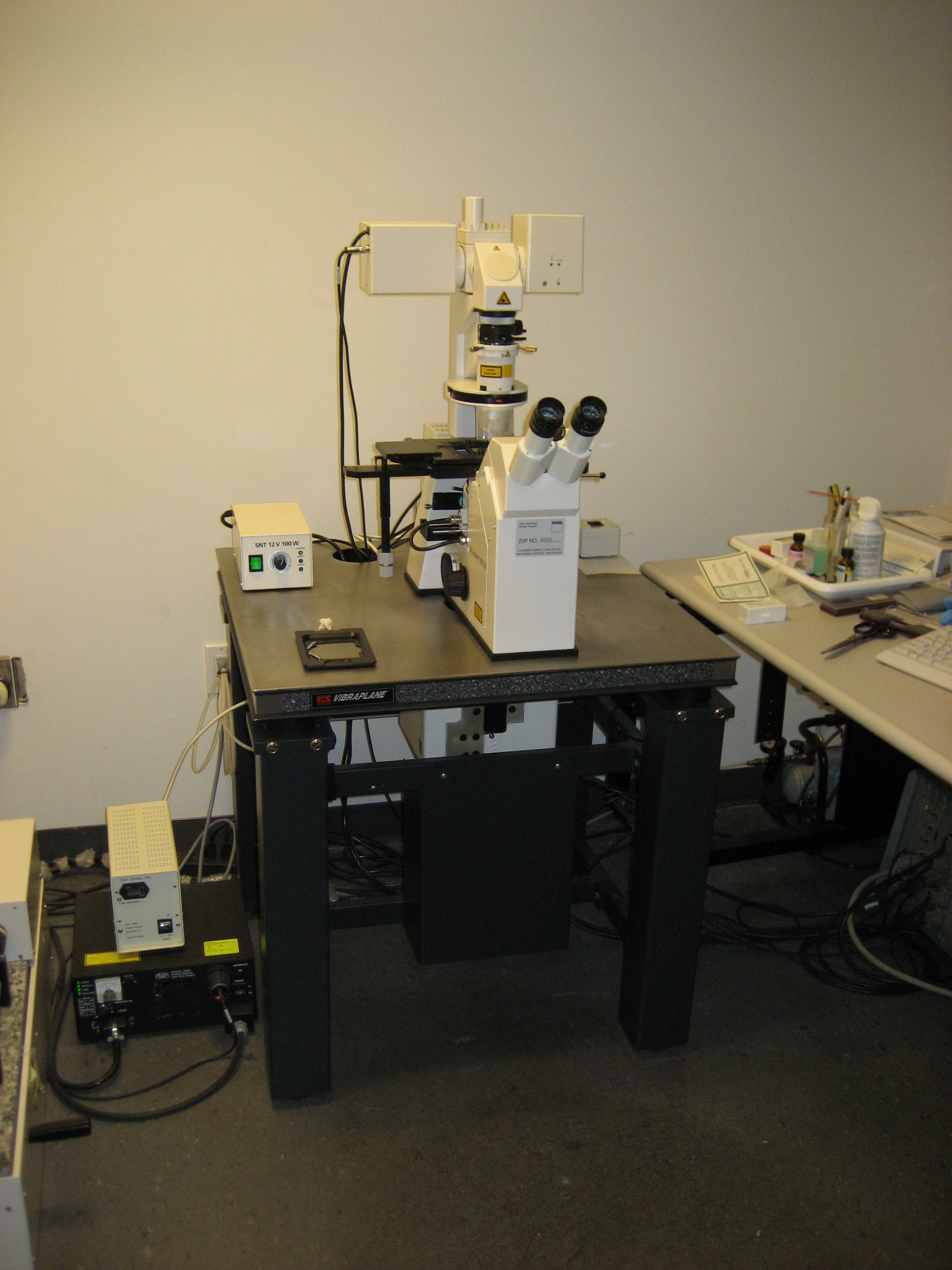
Figure 2 (right): The Zeiss Axiovert 100 at AMNH. The instrument is in a separate room
with support facilitites. A clean hood is used for sample preparation.
Back to:
top of this page
D.S. Ebel home
Earth and Planetary Sciences at A.M.N.H.
A.M.N.H. home
Last modified February 20, 2008